Covariate Adjustment in Randomized Trials
Josh Betz (jbetz@jhu.edu), Kelly Van Lancker (kvanlan3@jhu.edu), and Michael Rosenblum (mrosen@jhu.edu)
- Executive Summary
- Covariate Adjusted Analysis in Practice
- Chemotherapy for Stage B/C Colon Cancer
- Checks on the Data:
- Types of Tests & Estimators: Time-to-Event Outcomes
- Implementing Unadjusted Tests & Models
- Covariate Adjusted Analyses
- References
Executive Summary
Randomly allocating participants to treatment arms will tend to produce groups that are initially comparable to one another across both observed and unobserved factors. In any given randomized trial, there will be some degree of imbalance in the distribution of baseline covariates between treatment groups. When a variable is a strong predictor of the outcome and is imbalanced across treatment arms, it represents a potential confounding variable and source of bias, even if these differences are not statistically significant (Assmann et al. 2000). Confounding can be addressed both in the design phase of a trial, using stratified randomization to lessen the potential for imbalance, and in during the analysis phase, through covariate adjustment.
Covariate adjustment can lead to a more efficient trial, potentially lowering the required sample size to detect a given treatment effect if it exists, or provide greater precision (shorter confidence interval widths and higher power) for the same sample size and treatment effect. When stratified randomization is used, covariate adjustment is generally suggested, but not always implemented, which can lead to reduced power and precision (Kahan and Morris 2011). Accessible and practical discussions of baseline balance, stratified randomized trials, and adjusted analyses are also available to offer further explanation and guidance to investigators (Kernan 1999; Assmann et al. 2000).
When using regression models for inference, it is important to understand how model misspecification may affect statistical inference. Fortunately, there are several approaches to covariate-adjusted analyses whose validity does not depend on a correctly specified model, or provide inference with greater robustness to misspecification than those used in common practice.
The focus of this template is on the analysis of time-to-event outcomes. This tutorial illustrates the use of covariate-adjusted analysis in clinical trials using an example dataset from a randomized trial of treatments for colon cancer. This tutorial illustrates calculating the restricted mean survival time (RMST) and survival probability with and without adjustment for covariates. These methods are contrasted against methods commonly used in observational studies and randomized trials, such as the logrank test and Cox Proportional Hazards model.
Using This Tutorial
This tutorial contains an example dataset as well as code to illustrate how to perform covariate adjustment in practice for continuous and binary outcomes using R. R is a free and open source language and statistical computing environment. Rstudio is a powerful development environment for using the R language. The ability of R can be extended by downloading software packages from the Comprehensive R Archival Network (CRAN). In R, these packages can be installed from the Comprehensive R Archival Network, or CRAN, using the install.packages() command. In Rstudio IDE, there is a ‘Packages’ tab that allows users to see which packages are installed, which packages are currently in use, and install or update packages using a graphical interface. Once the required packages are installed, data can be downloaded from Github, and users can run the code on their own devices.
Covariate Adjusted Analysis in Practice
Once R and Rstudio have been installed, additional packages must be installed from CRAN or Github, and some tools may need to be installed to compile packages from source code.
Installing RTools - Compiling Packages from Source
Some R packages must be compiled from source code. RTools is a set of software tools for compiling such R packages. Choose the appropriate version of RTools for your version of R.
Installing R Packages from CRAN
The following packages and their dependencies needs to be installed:
- knitr - Tools for literate programming: including code in reproducible reports
- devtools - A suite of tools for R package development
- tidyverse - An ecosystem of packages for working with data
- table1 - Creating simple tabulations in aggregate and by treatment arm
- survminer - Creating plots of time-to-event data
- survRM2 - Calculating the restricted mean survival time (RMST) with and without covariate adjustment.
required_packages <-
  c("knitr",
    "devtools",
    "tidyverse",
    "table1",
    "survminer",
    "coxrobust",
    "survRM2"
  )

install.packages(required_packages)
NOTE: Packages only need to be installed once: after installation, they can be updated using the ‘Packages’ tab in RStudio.
Installing R Packages from GitHub
Github is a platform for developing software and documentation with version control. It is a common platform for R package development, testing, reporting and addressing software issues. Use devtools::install_github to install packages hosted on Github.
devtools::install_github("nt-williams/simul")
devtools::install_github("nt-williams/adjrct")
Loading Installed Packages
Once the required packages are installed, they can be loaded using library() command.
library(knitr) # Printing tables in reports
library(tidyverse) # Data manipulation: dplyr, tidyr
library(table1) # Creation of Summary tables
library(survival) # For AFT & Cox Proportional Hazards Models
library(survminer) # For Kaplan-Meier Plots
library(coxrobust) # For coxr: Robust Cox PH Model
library(survRM2) # For restricted mean survival times (RMST)
library(adjrct) # For TMLE estimates of RMST, Survival Probability
library(splines) # For adding smoothing splines
Chemotherapy for Stage B/C Colon Cancer
Data used in this example come from the survival::colon dataset, a trial of adjuvant chemotherapy for colon cancer. See ?survival::colon for more details. In brief, the study had three treatment arms: observation, levamisole, and levamisole + 5-Fluorouracil.
These data have been pre-processed to make the data more usable. Event times were converted from long (one row per event type: recurrence vs. death) to wide (each event as separate columns instead of rows), categorical variables were cast as factors with named labels to make them easier to interpret, and since some individuals were followed up for 8 years or so, the scale of time was coarsened to months instead of days. The code for processing the data is available here
id: Patient id- Baseline Covariates
arm: Treatment - Obs(ervation), Lev(amisole), Lev(amisole)+5-FUage: Age in yearssex: Patient Sexobstruction: obstruction of colon by tumorperforation: perforation of colonadherence: adherence to nearby organspositive_nodes: number of lymph nodes with detectable cancerdifferentiation: differentiation of tumor (1. Well,2. Moderate,3. Poor)extent: Extent of local spread (1. Submucosa,2. Muscle,3. Serosa,4. Contiguous structures)time_surgery_registration: time from surgery to registration
- Outcome:
event_recurrence: Observed (1) or Censored (0)time_to_recurrence: days until recurrence eventmonths_to_recurrence: months until recurrence eventevent_death: Observed (1) or Censored (0)time_to_death: days until recurrence eventmonths_to_death: months until recurrence eventevent_composite: Observed death OR recurrence (1) or neither event (0)time_to_composite: days until first composite event or censoring timemonths_to_composite: days until first composite event or censoring time
Since some functions require a binary treatment indicator and the study contains three arms, we can create a dataset for each binary treatment comparison of interest:
# Datasets with Binary Treatment ###############################################
# LEV vs Obs
colon_cancer_lev_vs_obs <-
  colon_cancer %>%
  dplyr::filter(
    arm %in% c("Lev", "Obs")
  ) %>%
  dplyr::mutate(
    tx = as.integer(1*(arm == "Lev"))
  )


# LEV+5FU vs LEV
colon_cancer_lev5fu_vs_lev <-
  colon_cancer %>%
  dplyr::filter(
    arm %in% c("Lev", "Lev+5FU")
  ) %>%
  dplyr::mutate(
    tx = as.integer(1*(arm == "Lev+5FU"))
  )


# LEV+5FU vs Obs
colon_cancer_lev5fu_vs_obs <-
  colon_cancer %>%
  dplyr::filter(
    arm %in% c("Obs", "Lev+5FU")
  ) %>%
  dplyr::mutate(
    tx = as.integer(1*(arm == "Lev+5FU"))
  )
Baseline Demographics & Stratum
Below are summary statistics of participant characteristics at baseline.
table1(
  ~ age + sex + obstruction + perforation + organ_adherence +
    differentiation + local_spread + time_surgery_registration +
    positive_nodes + recurrence + death + composite | arm,
  data = colon_cancer_original
)
| Obs (N=315) | Lev (N=310) | Lev+5FU (N=304) | Overall (N=929) | |
|---|---|---|---|---|
| age | ||||
| Mean (SD) | 59.5 (12.0) | 60.1 (11.6) | 59.7 (12.3) | 59.8 (11.9) |
| Median (Min, Max) | 60.0 (18.0, 85.0) | 61.0 (27.0, 83.0) | 62.0 (26.0, 81.0) | 61.0 (18.0, 85.0) |
| sex | ||||
| 0. Female | 149 (47.3%) | 133 (42.9%) | 163 (53.6%) | 445 (47.9%) |
| 1. Male | 166 (52.7%) | 177 (57.1%) | 141 (46.4%) | 484 (52.1%) |
| obstruction | ||||
| 0. No | 252 (80.0%) | 247 (79.7%) | 250 (82.2%) | 749 (80.6%) |
| 1. Yes | 63 (20.0%) | 63 (20.3%) | 54 (17.8%) | 180 (19.4%) |
| perforation | ||||
| 0. No | 306 (97.1%) | 300 (96.8%) | 296 (97.4%) | 902 (97.1%) |
| 1. Yes | 9 (2.9%) | 10 (3.2%) | 8 (2.6%) | 27 (2.9%) |
| organ_adherence | ||||
| 0. No | 268 (85.1%) | 261 (84.2%) | 265 (87.2%) | 794 (85.5%) |
| 1. Yes | 47 (14.9%) | 49 (15.8%) | 39 (12.8%) | 135 (14.5%) |
| differentiation | ||||
| 1. Well | 27 (8.6%) | 37 (11.9%) | 29 (9.5%) | 93 (10.0%) |
| 2. Moderate | 229 (72.7%) | 219 (70.6%) | 215 (70.7%) | 663 (71.4%) |
| 3. Poor | 52 (16.5%) | 44 (14.2%) | 54 (17.8%) | 150 (16.1%) |
| Missing | 7 (2.2%) | 10 (3.2%) | 6 (2.0%) | 23 (2.5%) |
| local_spread | ||||
| 1. Submucosa | 8 (2.5%) | 3 (1.0%) | 10 (3.3%) | 21 (2.3%) |
| 2. Muscle | 38 (12.1%) | 36 (11.6%) | 32 (10.5%) | 106 (11.4%) |
| 3. Serosa | 249 (79.0%) | 259 (83.5%) | 251 (82.6%) | 759 (81.7%) |
| 4. Contiguous structures | 20 (6.3%) | 12 (3.9%) | 11 (3.6%) | 43 (4.6%) |
| time_surgery_registration | ||||
| 0. Short | 224 (71.1%) | 230 (74.2%) | 228 (75.0%) | 682 (73.4%) |
| 1. Long | 91 (28.9%) | 80 (25.8%) | 76 (25.0%) | 247 (26.6%) |
| positive_nodes | ||||
| Mean (SD) | 3.79 (3.73) | 3.69 (3.56) | 3.49 (3.42) | 3.66 (3.57) |
| Median (Min, Max) | 2.00 (0, 27.0) | 2.00 (0, 33.0) | 2.00 (1.00, 24.0) | 2.00 (0, 33.0) |
| Missing | 3 (1.0%) | 6 (1.9%) | 9 (3.0%) | 18 (1.9%) |
| recurrence | ||||
| 0. No | 138 (43.8%) | 138 (44.5%) | 185 (60.9%) | 461 (49.6%) |
| 1. Yes | 177 (56.2%) | 172 (55.5%) | 119 (39.1%) | 468 (50.4%) |
| death | ||||
| 0. No | 147 (46.7%) | 149 (48.1%) | 181 (59.5%) | 477 (51.3%) |
| 1. Yes | 168 (53.3%) | 161 (51.9%) | 123 (40.5%) | 452 (48.7%) |
| composite | ||||
| 0. No | 125 (39.7%) | 128 (41.3%) | 170 (55.9%) | 423 (45.5%) |
| 1. Yes | 190 (60.3%) | 182 (58.7%) | 134 (44.1%) | 506 (54.5%) |
Note that differentiation and positive_nodes contain missing values, which must be imputed. If there are any missing covariates, observations may be dropped from analyses, or these may cause errors in other functions.
Below are summary statistics of participant characteristics at baseline after imputing missing baseline covariates.
table1(
  ~ age + sex + obstruction + perforation + organ_adherence +
    differentiation + local_spread + time_surgery_registration +
    positive_nodes + recurrence + death + composite | arm,
  data = colon_cancer
)
| Obs (N=315) | Lev (N=310) | Lev+5FU (N=304) | Overall (N=929) | |
|---|---|---|---|---|
| age | ||||
| Mean (SD) | 59.5 (12.0) | 60.1 (11.6) | 59.7 (12.3) | 59.8 (11.9) |
| Median (Min, Max) | 60.0 (18.0, 85.0) | 61.0 (27.0, 83.0) | 62.0 (26.0, 81.0) | 61.0 (18.0, 85.0) |
| sex | ||||
| 0. Female | 149 (47.3%) | 133 (42.9%) | 163 (53.6%) | 445 (47.9%) |
| 1. Male | 166 (52.7%) | 177 (57.1%) | 141 (46.4%) | 484 (52.1%) |
| obstruction | ||||
| 0. No | 252 (80.0%) | 247 (79.7%) | 250 (82.2%) | 749 (80.6%) |
| 1. Yes | 63 (20.0%) | 63 (20.3%) | 54 (17.8%) | 180 (19.4%) |
| perforation | ||||
| 0. No | 306 (97.1%) | 300 (96.8%) | 296 (97.4%) | 902 (97.1%) |
| 1. Yes | 9 (2.9%) | 10 (3.2%) | 8 (2.6%) | 27 (2.9%) |
| organ_adherence | ||||
| 0. No | 268 (85.1%) | 261 (84.2%) | 265 (87.2%) | 794 (85.5%) |
| 1. Yes | 47 (14.9%) | 49 (15.8%) | 39 (12.8%) | 135 (14.5%) |
| differentiation | ||||
| 1. Well | 27 (8.6%) | 37 (11.9%) | 29 (9.5%) | 93 (10.0%) |
| 2. Moderate | 235 (74.6%) | 228 (73.5%) | 220 (72.4%) | 683 (73.5%) |
| 3. Poor | 53 (16.8%) | 45 (14.5%) | 55 (18.1%) | 153 (16.5%) |
| local_spread | ||||
| 1. Submucosa | 8 (2.5%) | 3 (1.0%) | 10 (3.3%) | 21 (2.3%) |
| 2. Muscle | 38 (12.1%) | 36 (11.6%) | 32 (10.5%) | 106 (11.4%) |
| 3. Serosa | 249 (79.0%) | 259 (83.5%) | 251 (82.6%) | 759 (81.7%) |
| 4. Contiguous structures | 20 (6.3%) | 12 (3.9%) | 11 (3.6%) | 43 (4.6%) |
| time_surgery_registration | ||||
| 0. Short | 224 (71.1%) | 230 (74.2%) | 228 (75.0%) | 682 (73.4%) |
| 1. Long | 91 (28.9%) | 80 (25.8%) | 76 (25.0%) | 247 (26.6%) |
| positive_nodes | ||||
| Mean (SD) | 3.80 (3.74) | 3.71 (3.56) | 3.51 (3.41) | 3.68 (3.57) |
| Median (Min, Max) | 2.00 (0, 27.0) | 2.00 (0, 33.0) | 2.00 (1.00, 24.0) | 2.00 (0, 33.0) |
| recurrence | ||||
| 0. No | 138 (43.8%) | 138 (44.5%) | 185 (60.9%) | 461 (49.6%) |
| 1. Yes | 177 (56.2%) | 172 (55.5%) | 119 (39.1%) | 468 (50.4%) |
| death | ||||
| 0. No | 147 (46.7%) | 149 (48.1%) | 181 (59.5%) | 477 (51.3%) |
| 1. Yes | 168 (53.3%) | 161 (51.9%) | 123 (40.5%) | 452 (48.7%) |
| composite | ||||
| 0. No | 125 (39.7%) | 128 (41.3%) | 170 (55.9%) | 423 (45.5%) |
| 1. Yes | 190 (60.3%) | 182 (58.7%) | 134 (44.1%) | 506 (54.5%) |
Checks on the Data:
Frequency of Events
Rare events may lead to numerical instabilities in estimation: it is always advisable to check whether the frequencies of events in aggregate and within categories of interest are sufficient for the planned analysis. For example, tabulations can assess whether there are sufficient events within obstruction to support analysis:
table1(
  ~ recurrence + death + composite | differentiation:arm,
  data = colon_cancer,
  overall = NULL
)
| 1. Well | 2. Moderate | 3. Poor | |||||||
|---|---|---|---|---|---|---|---|---|---|
| Obs (N=27) | Lev (N=37) | Lev+5FU (N=29) | Obs (N=235) | Lev (N=228) | Lev+5FU (N=220) | Obs (N=53) | Lev (N=45) | Lev+5FU (N=55) | |
| recurrence | |||||||||
| 0. No | 10 (37.0%) | 19 (51.4%) | 20 (69.0%) | 109 (46.4%) | 101 (44.3%) | 138 (62.7%) | 19 (35.8%) | 18 (40.0%) | 27 (49.1%) |
| 1. Yes | 17 (63.0%) | 18 (48.6%) | 9 (31.0%) | 126 (53.6%) | 127 (55.7%) | 82 (37.3%) | 34 (64.2%) | 27 (60.0%) | 28 (50.9%) |
| death | |||||||||
| 0. No | 11 (40.7%) | 19 (51.4%) | 21 (72.4%) | 118 (50.2%) | 112 (49.1%) | 132 (60.0%) | 18 (34.0%) | 18 (40.0%) | 28 (50.9%) |
| 1. Yes | 16 (59.3%) | 18 (48.6%) | 8 (27.6%) | 117 (49.8%) | 116 (50.9%) | 88 (40.0%) | 35 (66.0%) | 27 (60.0%) | 27 (49.1%) |
| composite | |||||||||
| 0. No | 10 (37.0%) | 17 (45.9%) | 20 (69.0%) | 98 (41.7%) | 94 (41.2%) | 125 (56.8%) | 17 (32.1%) | 17 (37.8%) | 25 (45.5%) |
| 1. Yes | 17 (63.0%) | 20 (54.1%) | 9 (31.0%) | 137 (58.3%) | 134 (58.8%) | 95 (43.2%) | 36 (67.9%) | 28 (62.2%) | 30 (54.5%) |
Reference level for Treatment
When the treatment is a factor variable, we can use the levels() function to see the reference level (i.e. the comparator/control group): it will appear as the first level.
# Check reference level
levels(colon_cancer$arm)
## [1] "Obs" "Lev" "Lev+5FU"
Make sure that the reference level is appropriately chosen before running analyses to avoid errors in interpretation and inference.
Types of Tests & Estimators: Time-to-Event Outcomes
The Kaplan-Meier (K-M) estimate of the survival function is a ubiquitous approach to estimating and visualizing the survival probability, i.e. the probability of not having an event of interest, over a follow-up period. The K-M estimator assumes that censoring is independent of the event time within each treatment arm, which may be violated if certain baseline characteristics, such as disease severity, are associated with both the event time of interest and dropout (Dı́az et al. 2018). This could occur if individuals with greater baseline severity are more likely to have the event and more likely to drop out before the event is observed.
The logrank test is perhaps the most common method for performing sample size calculations and performing unadjusted comparisons of time-to-event outcomes. The logrank test is valid if censoring is independent of the treatment or independent of the event time in each treatment arm (Lancker, Dukes, and Vansteelandt 2021). The logrank test is most powerful under the proportional hazards assumption. When the proportional hazards assumption is violated, a weight function can be specified in a weighted logrank test to emphasize different domains of the survival curve. For more on the use of weighted logrank tests to address violations of the proportional hazards, see Lin and León (2017).
The Cox Proportional Hazards (PH) regression is the most common method for performing covariate-adjusted comparisons of time-to-event outcomes under the proportional hazards assumption. The logrank test is equivalent to the Score test in a Cox PH model which only includes a treatment indicator and no additional covariates. Inclusion of covariates allows relaxation of the uninformative censoring assumption, but raises concerns about the impact of model assumptions and specification.
The validity of tests for the hypothesis of no treatment effect in randomized experiments using the Cox PH model depends on the relationship of censoring times to the treatment assignment and covariates. If censoring times are conditionally independent of treatment assignment given the covariates, or conditionally independent of the covariates given the treatment assignment, tests are valid when the sandwich variance estimator is used. However, if the model is mispecified and the distribution of censoring times depends on both the treatment and covariates, tests based on the Cox model will not be valid, and alternatives should be considered (DiRienzo and Lagakos 2001).
When the proportional hazards assumption is violated, the estimates from a Cox PH model represent a weighted average of the hazard functions over time. The weights in this weighted average are determined by both the survival in each group and the censoring distribution. This dependence upon the censoring distribution makes it difficult to meaningfully interpret the estimate when there are appreciable violations of the PH assumption (Rudser, LeBlanc, and Emerson 2012).
Even in the situation when the proportional hazards assumption appears to hold, the clinical interpretation of the hazard ratio is not straightforward. In the absence of censoring, measures of a treatment effect are usually based on summaries of the outcome distribution that explicitly reference the scale of measurement of the outcome which facilitate evaluation of clinical importance, such as the mean, median, or proportion above or below a clinically meaningful threshold (Rudser, LeBlanc, and Emerson 2012). The hazard function is the instantaneous rate at which events occur, which changes over time, and does not quantify the expected length of time until the event (Rudser, LeBlanc, and Emerson 2012).
Since quantities such as survival probabilities (e.g. survival at 5 years), quantiles (e.g. median, 75th percentile), or the restricted mean survival time (RMST, e.g. average time without an event in the 5 yeras post randomization) explicitly reference the time frame of events, they may be more clinically meaningful for comparing treatments (Rudser, LeBlanc, and Emerson 2012). Survival probability and RMST are interpretable under violations of the proportional hazards assumption, and estimators for these quantities exist that are doubly robust (i.e. consistent if either the censoring or survival distributions are consistently estimated) and are at least as efficient as the K-M estimator (Dı́az et al. 2018).
While covariate-adjusted hazard ratios can be obtained from a Cox PH model, these are conditional treatment effects: they are the estimated hazard ratio given all of the covariates in the model. Covariate adjusted estimators of the survival probability and RMST are marginal treatment effects, which are useful for assessing the public health impact of an intervention on the intended use population. For more information on estimands and estimators for survival data, see the pages on estimands and estimators and models.
Implementing Unadjusted Tests & Models
Kaplan-Meier Survival Estimate: Death
KM for Death - Time Scale: Days
time_to_death_km <-
  survfit(
      formula = Surv(time_to_death, event_death) ~ arm,
      data = colon_cancer
    )

ggsurvplot(
  fit = time_to_death_km,
  conf.int = TRUE,
  risk.table = TRUE,
  surv.median.line = "hv",
  break.time.by = 365.25,
  xlab = "Days",
  ylab = "Overall survival probability"
)
KM for Death - Time Scale: Months
months_to_death_km <-
  survfit(
      formula = Surv(months_to_death, event_death) ~ arm,
      data = colon_cancer
    )

ggsurvplot(
  fit = months_to_death_km,
  conf.int = TRUE,
  risk.table = TRUE,
  surv.median.line = "hv",
  break.time.by = 12,
  xlab = "Months",
  ylab = "Overall survival probability"
)
Note that numbers at will not exactly match across plots: actual calendar months vary in length from 28 to 31 days, while the time scale is coarsened by periods of (365.25/12 $\approx$ 30.4) days.
KM for Death - Stratified by obstruction
ggsurvplot(
  fit = time_to_death_km,
  conf.int = TRUE,
  surv.median.line = "hv",
  break.time.by = 365,
  facet.by = "differentiation",
  xlab = "Days",
  ylab = "Overall survival probability"
) +
  theme(
    # Adjust Plot Labels for Readability
    axis.text.x = element_text(size = 18),
    axis.text.y = element_text(size = 18),
    axis.title.y = element_text(size = 26),
    axis.title.x = element_text(size = 26),
    strip.text = element_text(size = 26),
    legend.text = element_text(size = 22),
    legend.title = element_text(size = 22)
  )
Logrank Test
The logrank test (and the G-rho family of rank-based test procedures) can be obtained using survival::survdiff:
survival::survdiff(
  formula = Surv(months_to_death, event_death) ~ arm,
  data = colon_cancer
)
## Call:
## survival::survdiff(formula = Surv(months_to_death, event_death) ~
##     arm, data = colon_cancer)
##
##               N Observed Expected (O-E)^2/E (O-E)^2/V
## arm=Obs     315      168      148      2.56      3.86
## arm=Lev     310      161      146      1.51      2.26
## arm=Lev+5FU 304      123      157      7.50     11.65
##
##  Chisq= 11.7  on 2 degrees of freedom, p= 0.003
Cox Proportional Hazards Model
The Cox Proportional Hazards model can be fit using the survival::coxph function. Robust standard errors can be utilized with the argument robust = TRUE.
unadjusted_cox <-
  survival::coxph(
    formula = Surv(months_to_death, event_death) ~ arm,
    # Use Efron's Method for Tied Event Times
    ties = "efron",
    # Use Robust Standard Errors
    robust = TRUE,
    data = colon_cancer
  )

summary(unadjusted_cox)
## Call:
## survival::coxph(formula = Surv(months_to_death, event_death) ~
##     arm, data = colon_cancer, ties = "efron", robust = TRUE)
##
##   n= 929, number of events= 452
##
##                coef exp(coef) se(coef) robust se      z Pr(>|z|)
## armLev     -0.02658   0.97377  0.11030   0.10976 -0.242   0.8087
## armLev+5FU -0.37210   0.68929  0.11876   0.11857 -3.138   0.0017 **
## ---
## Signif. codes:  0 '***' 0.001 '**' 0.01 '*' 0.05 '.' 0.1 ' ' 1
##
##            exp(coef) exp(-coef) lower .95 upper .95
## armLev        0.9738      1.027    0.7853    1.2075
## armLev+5FU    0.6893      1.451    0.5463    0.8696
##
## Concordance= 0.536  (se = 0.013 )
## Likelihood ratio test= 12.18  on 2 df,   p=0.002
## Wald test            = 11.48  on 2 df,   p=0.003
## Score (logrank) test = 11.71  on 2 df,   p=0.003,   Robust = 12.11  p=0.002
##
##   (Note: the likelihood ratio and score tests assume independence of
##      observations within a cluster, the Wald and robust score tests do not).
Assuming the proportional hazards assumption is correct, the hazard of death in those receiving Lev+5FU was 31% lower ((1 - 0.68929) = 0.31071) than the observation arm.
The Proportional Hazards (PH) assumption can be assessed using survival::cox.zph:
unadjusted_cox_ph_test <- cox.zph(unadjusted_cox)

print(unadjusted_cox_ph_test)
##        chisq df    p
## arm     1.56  2 0.46
## GLOBAL  1.56  2 0.46
# Plot
plot(cox.zph(unadjusted_cox))
These plots should show an approximately constant value over time when the proportional hazards assumption holds.
Robust Cox Proportional Hazards Model
The coxrobust package has the coxr package for fitting a robust Cox proportional hazard model, based on a smooth modification of the partial likelihood (see ?coxrobust::coxr for details).
unadjusted_robust_cox <-
  coxr(
    formula = Surv(months_to_death, event_death) ~ arm,
    data = colon_cancer
  )

unadjusted_robust_cox_table <-
  with(unadjusted_robust_cox,
       data.frame(
         Beta = coefficients,
         SE = sqrt(diag(unadjusted_robust_cox$var))
       )
  ) %>%
  dplyr::mutate(
    `Beta LCL` = Beta + qnorm(p = 0.025)*SE,
    `Beta UCL` = Beta + qnorm(p = 0.0975)*SE,
    HR = exp(Beta),
    `HR LCL` = exp(`Beta LCL`),
    `HR UCL` = exp(`Beta UCL`)
  )

unadjusted_robust_cox_table %>%
  kable(
    x = .,
    digits = 2,
    caption = "Estimates from a Robust Cox Proportional Hazards Model."
  )
| Beta | SE | Beta LCL | Beta UCL | HR | HR LCL | HR UCL | |
|---|---|---|---|---|---|---|---|
| armLev | 0.04 | 0.14 | -0.23 | -0.14 | 1.04 | 0.80 | 0.87 |
| armLev+5FU | -0.29 | 0.14 | -0.57 | -0.47 | 0.75 | 0.57 | 0.62 |
Estimates from a Robust Cox Proportional Hazards Model.
Using the robust Cox PH model, the hazard of death in those receiving Lev+5FU was 25% lower ((1 - exp(-0.29)) = 0.2517364) than the observation arm. Alternatively, the hazard of death was 33% higher exp(-(-0.29)) = 1.336427 in the observation arm relative to the Lev+5FU arm.
Restricted Mean Survival Time: survRM2::rmst2
with(
  colon_cancer_lev5fu_vs_obs,
  survRM2::rmst2(
    time = months_to_death,
    status = event_death,
    arm = tx,
    tau = 60
  )
)
##
## The truncation time: tau = 60  was specified.
##
## Restricted Mean Survival Time (RMST) by arm
##                Est.    se lower .95 upper .95
## RMST (arm=1) 47.844 1.073    45.741    49.946
## RMST (arm=0) 44.241 1.087    42.110    46.372
##
##
## Restricted Mean Time Lost (RMTL) by arm
##                Est.    se lower .95 upper .95
## RMTL (arm=1) 12.156 1.073    10.054    14.259
## RMTL (arm=0) 15.759 1.087    13.628    17.890
##
##
## Between-group contrast
##                       Est. lower .95 upper .95     p
## RMST (arm=1)-(arm=0) 3.603     0.609     6.596 0.018
## RMST (arm=1)/(arm=0) 1.081     1.013     1.154 0.019
## RMTL (arm=1)/(arm=0) 0.771     0.619     0.961 0.020
The average survival time in the first 60 months was 47.84 months in the Lev+5FU arm and 44.24 months in the observation arm: the difference in average time without an event (RMST) between arms in the first 60 months was 3.6 months. The ratio of RMST between treatment and control was 1.081 (8% increase in RMST), and the mean difference in life expectancy lost to death (Restricted Mean Time Lost or RMTL) was 0.77 months.
Targeted Maximum Likelihood Estimator (TMLE): adjrct::survrct
The first step in using adjrct::survrct is to compute the metadata necessary for computing the model-robust estimates of restricted mean survival time and survival probability:
surv_metadata_unadj <-
  adjrct::survrct(
    outcome.formula = Surv(months_to_death, event_death) ~ tx,
    trt.formula = tx ~ 1,
    data = colon_cancer_lev5fu_vs_obs,
  )
Unadjusted Restricted Mean Survival Time (RMST)
adjrct::rmst(
  metadata = surv_metadata_unadj,
  horizon = 60
)
The average survival time in the first 60 months was 47.84 months in the Lev+5FU arm and 44.24 months in the observation arm: the difference in average time without an event between arms was 3.6 months.
Unadjusted Survival Probability
adjrct::survprob(
  metadata = surv_metadata_unadj,
  horizon = 60
)
The unadjusted survival probability in the first 60 months was 0.63 in the in the Lev+5FU arm and 0.53 in the observation arm. The difference in the probability of surviving the first 60 months between Lev+5FU and observation was 0.11 (i.e an 11% lower risk of dying in the first 60 months in the treatment arm relative to control).
Covariate Adjusted Analyses
Propensity Score
ps_model <-
  glm(
    formula =
      tx ~ age + positive_nodes +
      sex + obstruction + organ_adherence + differentiation +
      local_spread,
    data = colon_cancer_lev5fu_vs_obs,
    family = binomial(link = "logit")
  )

summary(ps_model)
##
## Call:
## glm(formula = tx ~ age + positive_nodes + sex + obstruction +
##     organ_adherence + differentiation + local_spread, family = binomial(link = "logit"),
##     data = colon_cancer_lev5fu_vs_obs)
##
## Deviance Residuals:
##    Min      1Q  Median      3Q     Max
## -1.350  -1.161  -0.876   1.186   1.533
##
## Coefficients:
##                                        Estimate Std. Error z value Pr(>|z|)
## (Intercept)                           0.3910622  0.6650025   0.588    0.556
## age                                   0.0005549  0.0067915   0.082    0.935
## positive_nodes                       -0.0253537  0.0234493  -1.081    0.280
## sex1. Male                           -0.2636635  0.1625075  -1.622    0.105
## obstruction1. Yes                    -0.1839938  0.2105093  -0.874    0.382
## organ_adherence1. Yes                -0.0957930  0.2446858  -0.391    0.695
## differentiation2. Moderate           -0.0783735  0.2876035  -0.273    0.785
## differentiation3. Poor                0.0577442  0.3371248   0.171    0.864
## local_spread2. Muscle                -0.2826257  0.5375651  -0.526    0.599
## local_spread3. Serosa                -0.0928858  0.4898133  -0.190    0.850
## local_spread4. Contiguous structures -0.6962111  0.6236855  -1.116    0.264
##
## (Dispersion parameter for binomial family taken to be 1)
##
##     Null deviance: 857.92  on 618  degrees of freedom
## Residual deviance: 849.83  on 608  degrees of freedom
## AIC: 871.83
##
## Number of Fisher Scoring iterations: 4
Adjusted Cox Proportional Hazards Model
adjusted_cox <-
  coxph(
    formula = Surv(months_to_death, event_death) ~ arm +
      # Covariates
      pspline(age) + pspline(positive_nodes) +
      sex + obstruction + organ_adherence + differentiation +
      local_spread,
    # Use Efron's Method for Tied Event Times
    ties = "efron",
    # Use Robust Standard Errors
    robust = TRUE,
    data = colon_cancer
  )
Assuming the proportional hazards assumption holds, conditioning on age, positive_nodes, sex, obstruction, organ_adherence, differentiation, and local_spread, the hazard of death in those receiving Lev+5FU was 33% lower ((1 - exp(-0.400301)) = 0.3298817) than the observation arm. Note that this is also a conditional treatment effect, not a marginal treatment effect.
cox.zph(
  fit = adjusted_cox
)
##                           chisq    df       p
## arm                      2.8385  1.99  0.2409
## pspline(age)             0.8629  4.08  0.9349
## pspline(positive_nodes)  5.1317  4.04  0.2791
## sex                      0.8663  1.00  0.3507
## obstruction              6.9092  0.99  0.0085
## organ_adherence          0.0808  1.00  0.7748
## differentiation         19.5067  1.99 5.7e-05
## local_spread             7.8919  2.99  0.0480
## GLOBAL                  42.3879 18.09  0.0010
Here we can see that obstruction, differentiation, and local_spread suggest departures from the proportional hazards assumption:
cox.zph(
  fit = adjusted_cox
) %>%
  plot(var = "differentiation")
abline(h = 0, col = rgb(1, 0, 0, 0.75))
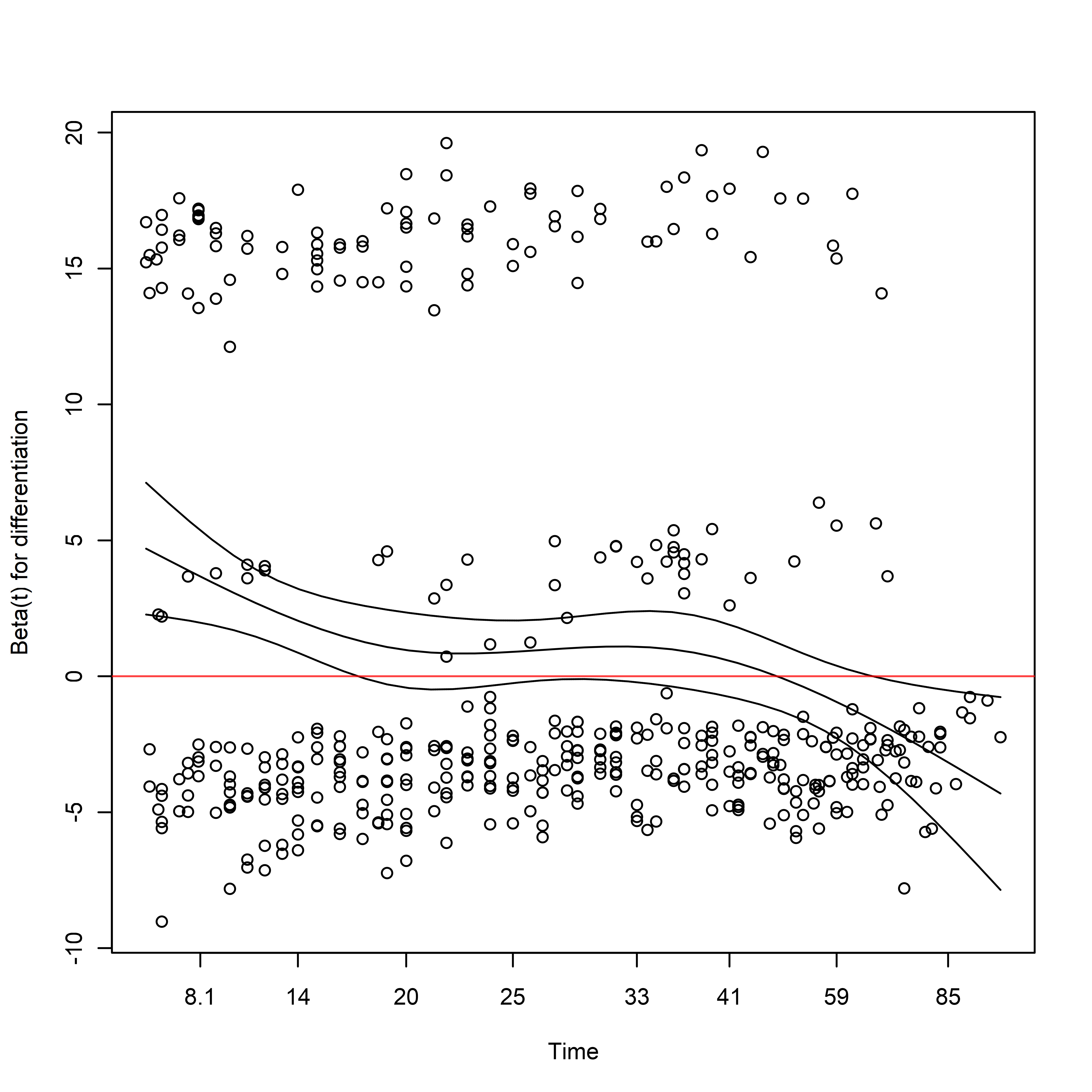
Note that the sign of the coefficient is initially large and positive, decreases with time, and eventually becomes negative in sign.
summary(adjusted_cox)
## Call:
## coxph(formula = Surv(months_to_death, event_death) ~ arm + pspline(age) +
##     pspline(positive_nodes) + sex + obstruction + organ_adherence +
##     differentiation + local_spread, data = colon_cancer, ties = "efron",
##     robust = TRUE)
##
##   n= 929, number of events= 452
##
##                           coef      se(coef) se2     Chisq DF   p
## armLev                    -0.040596 0.112021 0.11143  0.13 1.00 7.2e-01
## armLev+5FU                -0.400301 0.124375 0.12007 10.36 1.00 1.3e-03
## pspline(age), linear       0.006177 0.004094 0.00395  2.28 1.00 1.3e-01
## pspline(age), nonlin                                 11.47 3.08 1.0e-02
## pspline(positive_nodes),   0.052188 0.005713 0.02026 83.45 1.00 6.5e-20
## pspline(positive_nodes),                             57.99 3.04 1.7e-12
## sex1. Male                 0.025277 0.098304 0.09563  0.07 1.00 8.0e-01
## obstruction1. Yes          0.258930 0.122368 0.11708  4.48 1.00 3.4e-02
## organ_adherence1. Yes      0.168851 0.134919 0.12866  1.57 1.00 2.1e-01
## differentiation2. Moderat -0.111283 0.167590 0.16651  0.44 1.00 5.1e-01
## differentiation3. Poor     0.220141 0.203422 0.19335  1.17 1.00 2.8e-01
## local_spread2. Muscle      0.305089 0.532604 0.53042  0.33 1.00 5.7e-01
## local_spread3. Serosa      0.769705 0.514378 0.50684  2.24 1.00 1.3e-01
## local_spread4. Contiguous  1.196367 0.556507 0.54039  4.62 1.00 3.2e-02
##
##                           exp(coef) exp(-coef) lower .95 upper .95
## armLev                       0.9602    1.04143    0.7709    1.1960
## armLev+5FU                   0.6701    1.49227    0.5252    0.8551
## ps(age)3                     1.0212    0.97920    0.5947    1.7538
## ps(age)4                     1.0585    0.94473    0.3642    3.0762
## ps(age)5                     1.1263    0.88787    0.2515    5.0433
## ps(age)6                     1.1052    0.90480    0.1978    6.1750
## ps(age)7                     1.0070    0.99302    0.1755    5.7795
## ps(age)8                     0.9280    1.07758    0.1689    5.0983
## ps(age)9                     0.9912    1.00888    0.1852    5.3061
## ps(age)10                    1.2091    0.82708    0.2260    6.4672
## ps(age)11                    1.2763    0.78353    0.2373    6.8635
## ps(age)12                    1.3184    0.75851    0.2395    7.2571
## ps(age)13                    1.6505    0.60589    0.2636   10.3356
## ps(age)14                    2.1013    0.47589    0.2616   16.8807
## ps(positive_nodes)3          2.0606    0.48530    1.4253    2.9791
## ps(positive_nodes)4          4.4107    0.22672    2.2495    8.6481
## ps(positive_nodes)5          8.0308    0.12452    4.1120   15.6842
## ps(positive_nodes)6          9.3855    0.10655    5.1010   17.2688
## ps(positive_nodes)7         10.4631    0.09557    5.4463   20.1009
## ps(positive_nodes)8         11.1372    0.08979    5.2307   23.7132
## ps(positive_nodes)9         11.9044    0.08400    5.2776   26.8521
## ps(positive_nodes)10        13.0534    0.07661    5.7741   29.5095
## ps(positive_nodes)11        13.0080    0.07688    6.0309   28.0567
## ps(positive_nodes)12        11.7280    0.08527    5.7361   23.9790
## ps(positive_nodes)13        10.0577    0.09943    4.8663   20.7875
## ps(positive_nodes)14         8.5537    0.11691    3.7527   19.4965
## sex1. Male                   1.0256    0.97504    0.8459    1.2435
## obstruction1. Yes            1.2955    0.77188    1.0193    1.6467
## organ_adherence1. Yes        1.1839    0.84463    0.9088    1.5423
## differentiation2. Moderat    0.8947    1.11771    0.6442    1.2426
## differentiation3. Poor       1.2463    0.80241    0.8365    1.8568
## local_spread2. Muscle        1.3567    0.73706    0.4777    3.8535
## local_spread3. Serosa        2.1591    0.46315    0.7878    5.9172
## local_spread4. Contiguous    3.3081    0.30229    1.1114    9.8464
##
## Iterations: 5 outer, 14 Newton-Raphson
##      Theta= 0.89032
##      Theta= 0.8243073
## Degrees of freedom for terms= 2.0 4.1 4.0 1.0 1.0 1.0 2.0 3.0
## Concordance= 0.68  (se = 0.012 )
## Likelihood ratio test= 159.9  on 18.09 df,   p=<2e-16
Adjusted Robust Cox Proportional Hazards Model
adjusted_robust_cox <-
  coxr(
    formula = Surv(months_to_death, event_death) ~ arm +
      # Covariates
      bs(age) + bs(positive_nodes) +
      sex + obstruction + organ_adherence + differentiation +
      local_spread,
    data = colon_cancer
  )

adjusted_robust_cox_table <-
  with(adjusted_robust_cox,
       data.frame(
         Beta = coefficients,
         SE = sqrt(diag(unadjusted_robust_cox$var))
       )
  ) %>%
  dplyr::mutate(
    `Beta LCL` = Beta + qnorm(p = 0.025)*SE,
    `Beta UCL` = Beta + qnorm(p = 0.0975)*SE,
    HR = exp(Beta),
    `HR LCL` = exp(`Beta LCL`),
    `HR UCL` = exp(`Beta UCL`)
  )

adjusted_robust_cox_table %>%
  kable(
    x = .,
    digits = 2,
    caption = "Estimates from a Robust Cox Proportional Hazards Model."
  )
| Beta | SE | Beta LCL | Beta UCL | HR | HR LCL | HR UCL | |
|---|---|---|---|---|---|---|---|
| armLev | 0.00 | 0.14 | -0.27 | -0.18 | 1.00 | 0.76 | 0.84 |
| armLev+5FU | -0.30 | 0.14 | -0.58 | -0.48 | 0.74 | 0.56 | 0.62 |
| bs(age)1 | 0.15 | 0.14 | -0.11 | -0.02 | 1.16 | 0.89 | 0.98 |
| bs(age)2 | -0.74 | 0.14 | -1.01 | -0.92 | 0.48 | 0.36 | 0.40 |
| bs(age)3 | 1.03 | 0.14 | 0.77 | 0.86 | 2.80 | 2.15 | 2.35 |
| bs(positive_nodes)1 | 3.95 | 0.14 | 3.67 | 3.77 | 52.06 | 39.40 | 43.30 |
| bs(positive_nodes)2 | 1.20 | 0.14 | 0.94 | 1.03 | 3.33 | 2.56 | 2.80 |
| bs(positive_nodes)3 | 1.33 | 0.14 | 1.05 | 1.15 | 3.79 | 2.87 | 3.15 |
| sex1. Male | -0.01 | 0.14 | -0.27 | -0.18 | 0.99 | 0.76 | 0.83 |
| obstruction1. Yes | 0.44 | 0.14 | 0.16 | 0.26 | 1.56 | 1.18 | 1.29 |
| organ_adherence1. Yes | 0.20 | 0.14 | -0.07 | 0.02 | 1.22 | 0.94 | 1.02 |
| differentiation2. Moderate | -0.14 | 0.14 | -0.42 | -0.33 | 0.87 | 0.66 | 0.72 |
| differentiation3. Poor | 0.47 | 0.14 | 0.20 | 0.29 | 1.59 | 1.22 | 1.34 |
| local_spread2. Muscle | 0.15 | 0.14 | -0.13 | -0.04 | 1.16 | 0.88 | 0.96 |
| local_spread3. Serosa | 0.77 | 0.14 | 0.51 | 0.60 | 2.17 | 1.66 | 1.82 |
| local_spread4. Contiguous structures | 1.52 | 0.14 | 1.24 | 1.34 | 4.59 | 3.47 | 3.82 |
Estimates from a Robust Cox Proportional Hazards Model.
Assuming the proportional hazards assumption holds, conditioning on age, positive_nodes, sex, obstruction, organ_adherence, differentiation, and local_spread, the hazard of death in those receiving Lev+5FU was 26% lower ((1 - exp(-0.30)) = 0.2591818) than the observation arm using the robust Cox PH model. Note that this is also a conditional treatment effect, not a marginal treatment effect.
Targeted Maximum Likelihood
surv_metadata_adj <-
  adjrct::survrct(
    outcome.formula = Surv(months_to_death, event_death) ~ tx +
      age + positive_nodes +
      sex + obstruction + organ_adherence + differentiation +
      local_spread,
    trt.formula =
      tx ~ age + positive_nodes +
      sex + obstruction + organ_adherence + differentiation +
      local_spread,
    data = colon_cancer_lev5fu_vs_obs
  )
Calculate Restricted Mean Survival Time
rmst_metadata_adj <-
  adjrct::rmst(
    metadata = surv_metadata_adj,
    horizon = 60
  )

rmst_metadata_adj
## RMST Estimator: tmle

## Marginal RMST: E(min[T, 60] | A = a)

## Treatment Arm

## Estimate: 47.74

## Std. error: 1.07

## 95% CI: (45.64, 49.85)

## Control Arm

## Estimate: 44.53

## Std. error: 1.03

## 95% CI: (42.52, 46.54)

## Treatment Effect: E(min[T, 60] | A = 1) - E(min[T, 60] | A = 0)

## Additive effect

## Estimate: 3.22

## Std. error: 1.43

## 95% CI: (0.41, 6.02)
The covariate-adjusted average survival time in the first 60 months was 47.74 months in the Lev+5FU arm and 44.53 months in the observation arm: the difference in average time without an event between arms was 3.2 months. While the point estimates are similar to the unadjusted estimate, the variance of the estimate is reduced by about 13%: $1 - ({SE}{Unadj}/{SE}{Adj})^{2}$ = 1 - (1.43/1.53)^2 = 0.1264471.
rmst_metadata_adj_table <-
  with(
    rmst_metadata_adj$estimates[[1]],

    bind_rows(
      data.frame(
        Arm = "Treatment",
        Estimate = arm1,
        SE = arm1.std.error,
        LCL = arm1.conf.low,
        UCL = arm1.conf.high
      ),

      data.frame(
        Arm = "Control",
        Estimate = arm0,
        SE = arm0.std.error,
        LCL = arm0.conf.low,
        UCL = arm0.conf.high
      ),
      data.frame(
        Arm = "Treatment - Control",
        Estimate = theta,
        SE = std.error,
        LCL = theta.conf.low,
        UCL = theta.conf.high
      )
    )
  )

kable(
  x = rmst_metadata_adj_table,
  caption = "TMLE covariate-adjusted estimates of Restricted Mean Survival Time.",
  digits = 2
)
| Arm | Estimate | SE | LCL | UCL |
|---|---|---|---|---|
| Treatment | 47.74 | 1.07 | 45.64 | 49.85 |
| Control | 44.53 | 1.03 | 42.52 | 46.54 |
| Treatment - Control | 3.22 | 1.43 | 0.41 | 6.02 |
TMLE covariate-adjusted estimates of Restricted Mean Survival Time.
Calculate Survival Probability
survival_metadata_adj <-
  adjrct::survprob(
    metadata = surv_metadata_adj,
    horizon = 60
  )
## Warning: step size truncated due to increasing deviance

## Warning: step size truncated due to increasing deviance

## Warning: step size truncated due to increasing deviance
survival_metadata_adj
## Survival Probability Estimator: tmle

## Marginal Survival Probability: Pr(T > 60 | A = a)

## Treatment Arm

## Estimate: 0.63

## Std. error: 0.03

## 95% CI: (0.58, 0.69)

## Control Arm

## Estimate: 0.53

## Std. error: 0.03

## 95% CI: (0.48, 0.59)

## Treatment Effect: Pr(T > 60 | A = 1) - Pr(T > 60 | A = 0)

## Additive effect

## Estimate: 0.1

## Std. error: 0.04

## 95% CI: (0.03, 0.17)
The covariate-adjusted survival probability in the first 60 months was 0.63 in the in the Lev+5FU arm and 0.53 in the observation arm. The difference in the probability of surviving the first 60 months between Lev+5FU and observation was 0.10 (i.e an 10% lower risk of dying in the first 60 months in the treatment arm relative to control). The point estimates and variance estimates are almost identical to the unadjusted estimates.
survival_metadata_adj_table <-
  with(
    survival_metadata_adj$estimates[[1]],

    bind_rows(
      data.frame(
        Arm = "Treatment",
        Estimate = arm1,
        SE = arm1.std.error,
        LCL = arm1.conf.low,
        UCL = arm1.conf.high
      ),

      data.frame(
        Arm = "Control",
        Estimate = arm0,
        SE = arm0.std.error,
        LCL = arm0.conf.low,
        UCL = arm0.conf.high
      ),
      data.frame(
        Arm = "Treatment - Control",
        Estimate = theta,
        SE = std.error,
        LCL = theta.conf.low,
        UCL = theta.conf.high
      )
    )
  )

kable(
  x = survival_metadata_adj_table,
  caption = "TMLE covariate-adjusted estimates of survival probability.",
  digits = 2
)
| Arm | Estimate | SE | LCL | UCL |
|---|---|---|---|---|
| Treatment | 0.63 | 0.03 | 0.58 | 0.69 |
| Control | 0.53 | 0.03 | 0.48 | 0.59 |
| Treatment - Control | 0.10 | 0.04 | 0.03 | 0.17 |
TMLE covariate-adjusted estimates of survival probability.