1. Planning Information Monitored Designs with `impart` • impart

library(impart)
library(pwr) # Only required for examples, not for `impart`

Planning The Study

Planning information-monitored study is similar in many respects to planning a fixed-sample size study. Investigators decide on an effect size that is meaningful in magnitude, and decide on the appropriate Type I Error Rate, statistical power, and direction of alternatives of interest:

# Universal Study Design Parameters
minimum_difference <- 5 # Effect Size: Difference in Means of 5 or greater
alpha <- 0.05 # Type I Error Rate
power <- 0.9 # Statistical Power
test_sides <- 2 # Direction of Alternatives

The amount of data that must be collected depends on the amount of the information in the accruing data, with the information depending on the patterns of associations among variables, variability in the outcomes of interest, and degree of missingness. Such information is not always available when studies are being planned in practice.

Fixed sample size designs require investigators make assumptions about the factors affecting precision: when such assumptions are incorrect, studies can be over- or under-powered. Rather than planning data collection until a pre-specified sample size is reached, an information-monitored study continues data collection until the data collected provide enough precision to identify a meaningful difference with appropriate power and control of Type I Error.

Determining the Target Information Level

The information or precision required to achieve power $(1 - \beta)$ to identify a treatment effect $\delta$ with an $s$ -sided test with type I error rate $\alpha$ at the final analysis is given by:

$\mathcal{I}_{F} = \left(\frac{Z_{\alpha/s} + Z_{\beta}}{\delta}\right)^2 \approx \frac{1}{\left(SE(\hat{\delta})\right)^2} = \frac{1}{Var(\hat{\delta})}$

# Determine information required to achieve desired power at fixed error rate
information_single_stage <-
  impart::required_information_single_stage(
    delta = minimum_difference,
    alpha = alpha,
    power = power
  )

information_single_stage
#> [1] 0.4202969

For example, detecting a difference in means of 5 with 90% power and a Type I Error rate of 0.05 using a 2-sided test requires an information level of 0.4202969. Investigators can collect data until the precision (the reciprocal of the square of the standard error) reaches this level, and their analysis will have the appropriate power and Type I error control.

Translating Information into Sample Size

Translating information levels to a sample size requires making some assumption about nuisance parameters, such as the variability of the outcomes in each treatment arm. The information_to_n_continuous_1_to_1 function takes an information level and values of the nuisance parameters, and gives an approximate sample size. Note that this calculation only takes into account the information contained in the observed outcomes: if some outcomes are missing, or if the analysis makes use of information in baseline covariates and intermediate outcomes, this can change the sample size at which the target information level is reached.

# Assume Equal Variances: 7.5
approximate_n_sd_7.5 <-
  impart::information_to_n_continuous_1_to_1(
    information = information_single_stage,
    sigma_0 = 7.5,
    sigma_1 = 7.5,
    round_up = TRUE
  )
approximate_n_sd_7.5
#>   n_per_arm n_total
#> 1        48      96

# Compute Power: Fixed Sample Size
pwr::pwr.t.test(
  d = minimum_difference/7.5,
  sig.level = alpha,
  power = power
)
#> 
#>      Two-sample t test power calculation 
#> 
#>               n = 48.26427
#>               d = 0.6666667
#>       sig.level = 0.05
#>           power = 0.9
#>     alternative = two.sided
#> 
#> NOTE: n is number in *each* group
# Equal Variances: 10
approximate_n_sd_10 <-
  impart::information_to_n_continuous_1_to_1(
    information = information_single_stage,
    sigma_0 = 10,
    sigma_1 = 10,
    round_up = TRUE
  )
approximate_n_sd_10
#>   n_per_arm n_total
#> 1        85     170
# Compute Power: Fixed Sample Size
pwr::pwr.t.test(
  d = minimum_difference/10,
  sig.level = alpha,
  power = power
)
#> 
#>      Two-sample t test power calculation 
#> 
#>               n = 85.03128
#>               d = 0.5
#>       sig.level = 0.05
#>           power = 0.9
#>     alternative = two.sided
#> 
#> NOTE: n is number in *each* group

Note that under specific assumptions about the standard deviations in the populations are met, the sample size requirements determined using a fixed sample size design (pwr::pwr.t.test) or an information-monitored design (information_to_n_continuous_1_to_1) are the same. The advantage of an information-adaptive design is the sample size adapts to the information in the accruing data: rather than making assumptions about the standard deviations in each population, which could result in an over- or under-powered trial, data collection proceeds until the target information level is met, which ensures adequate power and Type I Error control.

Sequential Analyses in Studies

If the true effect of interest is greater than the minimum meaningful effect $\delta$ , the study may still be overpowered. Conversely, if the true effect is very small, or indicates that the benefits of participating in the study are not commensurate with risks, it may be futile to continue data collection. In such cases, interim analyses of the data can be used to guide more ethical, cost-effective data collection.

Group-Sequential Designs allow investigators to control Type I Error rates when performing pre-specified interim assessments of the differences between groups. Studies can also be stopped early for futility if accruing data suggest that a treatment is ineffective or harmful. The number and timing of analyses must be pre-specified, as well as the rules for stopping for efficacy and futility. The stopping rules are specified using ‘spending functions:’ alpha spending functions define efficacy stopping rules, and beta spending functions define futility stopping rules. For more information on group sequential designs, see the documentation for the RPACT package. This example will utilize the O’Brien-Fleming stopping rules for efficacy and futility.

In contrast to a group sequential design, which performs analyses at pre-specified fractions of the final sample size, an information-monitored study performs analyses when the data collected provide enough precision to identify a treatment effect with the appropriate power and Type I Error. Analyses are conducted when the precision reaches pre-specified fractions of this level of precision.

# Group Sequential Design Parameters
information_rates <-
  c(0.50, 0.75, 1.00) # Analyses at 50%, 75%, and 100% of the Total Information
type_of_design <- "asOF" # O'Brien-Fleming Alpha Spending
type_beta_spending <- "bsOF" # O'Brien-Fleming Beta Spending

The getDesignGroupSequential function in the rpact library can be used to specify the appropriate study design. For example, a two-sided test comparing $H_{0}: \mu_{T} - \mu_{C} = \delta_{0}$ vs. $H_{A}: \mu_{T} - \mu_{C} \neq \delta_{0}$

# Set up group sequential testing procedure
trial_design <-
  rpact::getDesignGroupSequential(
    alpha = alpha,
    beta = 1 - power,
    sided = 2,
    informationRates = information_rates,
    typeOfDesign = type_of_design,
    typeBetaSpending = type_beta_spending,
    bindingFutility = FALSE
  )

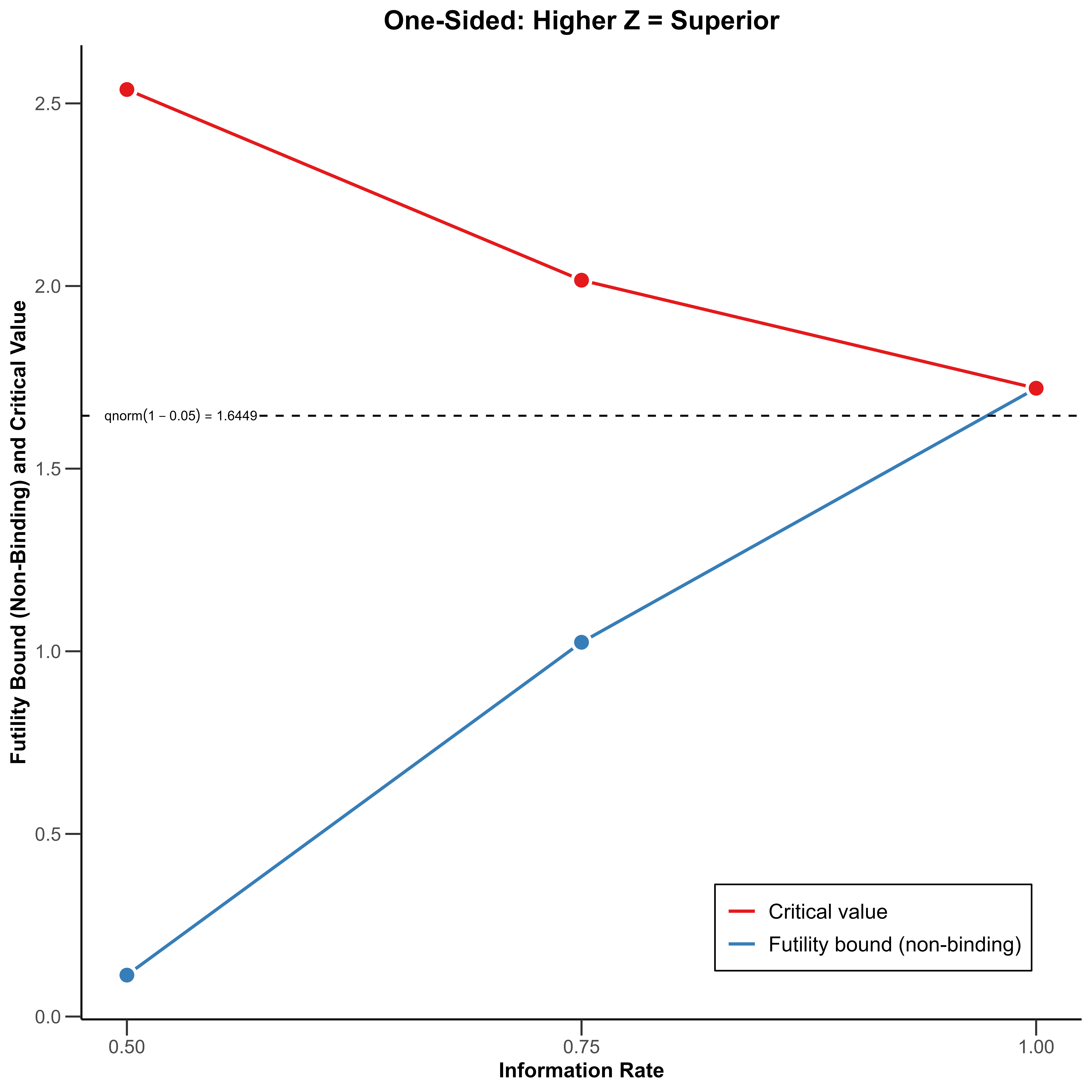
For a one-sided test using RPACT, the default boundaries assume users are testing $H_{0}: \mu_{T} - \mu_{C} < \delta_{0}$ vs. $H_{A}: \mu_{T} - \mu_{C} \ge \delta_{0}$ :

# One sided test: Higher values = Better
trial_design_one_sided_upper <-
  rpact::getDesignGroupSequential(
    alpha = alpha,
    beta = 1 - power,
    sided = 1,
    informationRates = information_rates,
    typeOfDesign = type_of_design,
    typeBetaSpending = type_beta_spending,
    bindingFutility = FALSE
  )

plot(
  trial_design_one_sided_upper,
  main = "One-Sided: Higher Z = Superior"
)

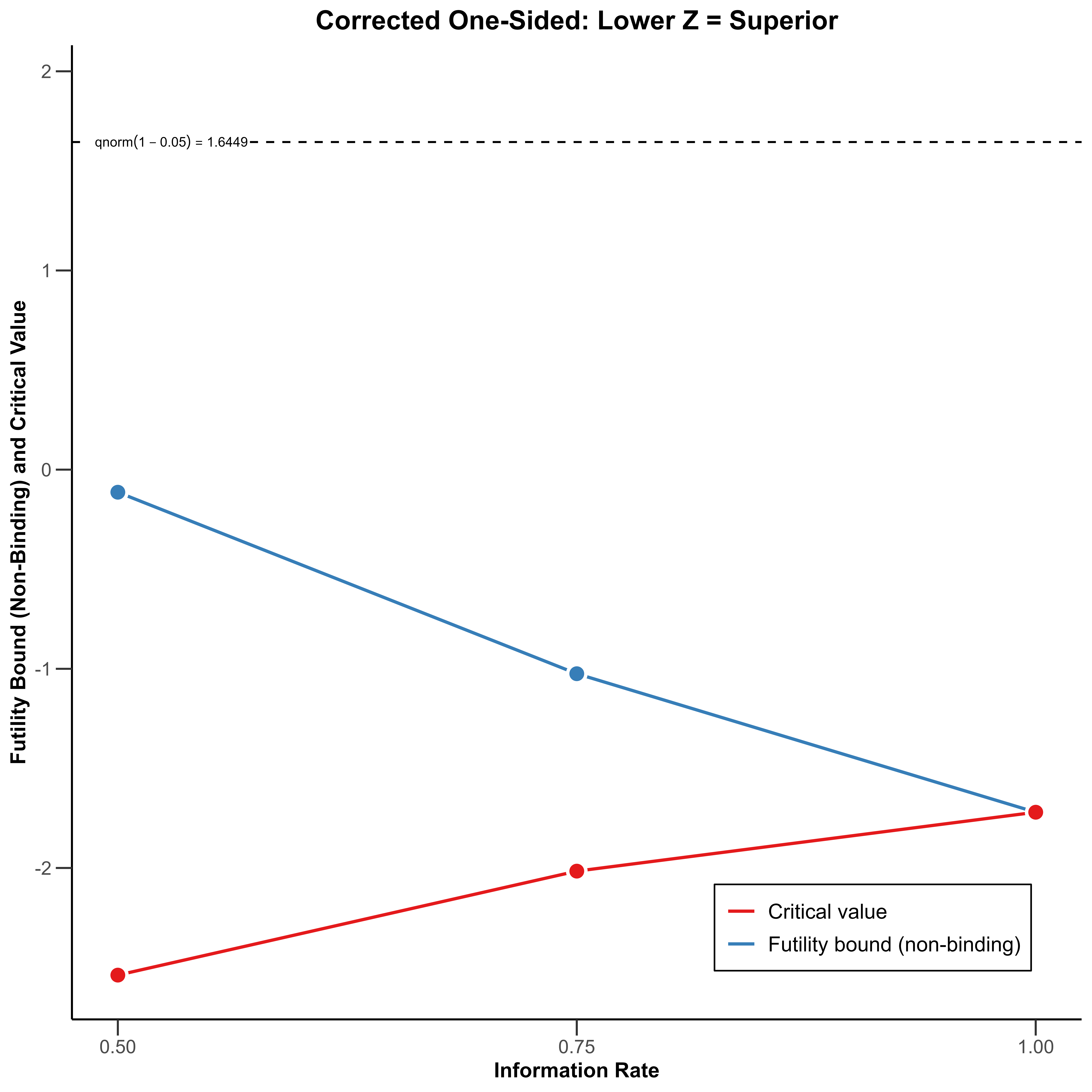
Users must must manually correct the resulting design boundaries to test $H_{0}: \mu_{T} - \mu_{C} > \delta_{0}$ vs. $H_{A}: \mu_{T} - \mu_{C} \le \delta_{0}$ . Until this correction is made, correct_one_sided_gsd() should be called on the result, which corrects the futility and efficacy boundaries:

trial_design_one_sided_lower <-
  correct_one_sided_gsd(
    trial_design = trial_design_one_sided_upper,
    higher_better = FALSE
  )

plot(
  trial_design_one_sided_lower,
  main = "Corrected One-Sided: Lower Z = Superior"
)

Once this issue is resolved, users can specify the direction using the directionUpper argument in other RPACT functions:

directionUpper = TRUE tests $H_{0}: \mu_{T} - \mu_{C} < \delta_{0}$ vs. $H_{A}: \mu_{T} - \mu_{C} \ge \delta_{0}$
directionUpper = FALSE tests $H_{0}: \mu_{T} - \mu_{C} > \delta_{0}$ vs. $H_{A}: \mu_{T} - \mu_{C} \le \delta_{0}$

# One sided test: Higher values = Better
trial_design_one_sided_higher <-
  rpact::getDesignGroupSequential(
    alpha = alpha,
    beta = 1 - power,
    sided = 1,
    informationRates = information_rates,
    typeOfDesign = type_of_design,
    typeBetaSpending = type_beta_spending,
    bindingFutility = FALSE,
    directionUpper = FALSE
  )

# One sided test: Lower values = Better
trial_design_one_sided_lower <-
  rpact::getDesignGroupSequential(
    alpha = alpha,
    beta = 1 - power,
    sided = 1,
    informationRates = information_rates,
    typeOfDesign = type_of_design,
    typeBetaSpending = type_beta_spending,
    directionUpper = TRUE
  )

Adjusting Information for Multiple Analyses

When doing sequential analyses in an information-monitored design, the target level of information must be adjusted:

# Inflate information level to account for multiple testing
information_adaptive <-
  impart::required_information_sequential(
    information_single_stage = information_single_stage,
    trial_design = trial_design
  )
information_adaptive
#> [1] 0.4558286

The information required under the specified design is 0.4558286, which is scaled up by the inflation factor mentioned in the summary of the design (1.0845394). This can be retrieved using rpact::getDesignCharacteristics(trial_design).

Including Covariate Information

Appropriately including information from covariates has the potential to increase the precision of analyses, meaning that target information levels can be reached at lower sample sizes, resulting in studies with shorter duration.

# Information Only From Final Outcomes
impart::information_to_n_continuous_1_to_1(
    information = information_rates*information_adaptive,
    sigma_0 = 10,
    sigma_1 = 10,
    round_up = FALSE
  )
#>   information sigma_0 sigma_1 n_per_arm   n_total
#> 1   0.2279143      10      10  45.58286  91.16572
#> 2   0.3418714      10      10  68.37429 136.74858
#> 3   0.4558286      10      10  91.16572 182.33143
# 10% Relative Efficiency Increase from Covariates
relative_efficiency <- 1.1
# Information From Final Outcomes + Covariates
impart::information_to_n_continuous_1_to_1(
  information = information_rates*information_adaptive/relative_efficiency,
  sigma_0 = 10,
  sigma_1 = 10,
  round_up = TRUE
)
#>   information sigma_0 sigma_1 n_per_arm n_total
#> 1   0.2071948      10      10        42      84
#> 2   0.3107922      10      10        63     126
#> 3   0.4143896      10      10        83     166
# 20% Relative Efficiency Increase from Covariates
relative_efficiency <- 1.2
# Information From Final Outcomes + Covariates
impart::information_to_n_continuous_1_to_1(
  information = information_rates*information_adaptive/relative_efficiency,
  sigma_0 = 10,
  sigma_1 = 10,
  round_up = TRUE
)
#>   information sigma_0 sigma_1 n_per_arm n_total
#> 1   0.1899286      10      10        38      76
#> 2   0.2848929      10      10        57     114
#> 3   0.3798572      10      10        76     152

The increase in precision from covariate adjustment is never known precisely during the planning of a study. Instead of relying on an assumption about the gain in precision from covariates, investigators can use information monitoring to adapt data collection to the accruing information from both covariates and outcomes.

Encapsulating Study Design

A monitored_design object encapsulates all of the information about an information monitored study that should be fixed at the outset, including the number of analyses, the information fractions at which analyses are conducted, the target level of information, the null value of the estimand of interest, the maximum feasible sample size, and the pseudorandom number generator seed which is used for analyses.

# Initialize the monitored design
monitored_design <-
  initialize_monitored_design(
    trial_design = trial_design,
    null_value = 0,
    maximum_sample_size = 280,
    information_target = information_adaptive,
    orthogonalize = TRUE,
    rng_seed_analysis = 54321
  )

monitored_design
#> $original_design
#> $original_design$trial_design
#> *Design parameters and output of group sequential design*
#> 
#> *User defined parameters*
#> 
#> * *Type of design*: O'Brien & Fleming type alpha spending 
#> * *Information rates*: 0.500, 0.750, 1.000 
#> * *Significance level*: 0.0500 
#> * *Type II error rate*: 0.1000 
#> * *Test*: two-sided 
#> * *Type of beta spending*: O'Brien & Fleming type beta spending 
#> 
#> *Derived from user defined parameters*
#> 
#> * *Maximum number of stages*: 3 
#> 
#> *Default parameters*
#> 
#> * *Stages*: 1, 2, 3 
#> * *Two-sided power*: FALSE 
#> * *Binding futility*: FALSE 
#> * *Beta adjustment*: TRUE 
#> * *Tolerance*: 1e-08 
#> 
#> *Output*
#> 
#> * *Power*: 0.2825, 0.7164, 0.9000 
#> * *Futility bounds (non-binding)*: 0.387, 1.282 
#> * *Cumulative alpha spending*: 0.003051, 0.019299, 0.050000 
#> * *Cumulative beta spending*: 0.02001, 0.05752, 0.10000 
#> * *Critical values*: 2.963, 2.359, 2.014 
#> * *Stage levels (one-sided)*: 0.001525, 0.009162, 0.022000 
#> 
#> 
#> $original_design$maximum_sample_size
#> [1] 280
#> 
#> $original_design$null_value
#> [1] 0
#> 
#> $original_design$information_target
#> [1] 0.4558286
#> 
#> $original_design$orthogonalize
#> [1] TRUE
#> 
#> $original_design$rng_seed_analysis
#> [1] 54321
#> 
#> $original_design$information_fractions
#> [1] 0.50 0.75 1.00
#> 
#> $original_design$information_thresholds
#> [1] 0.2279143 0.3418714 0.4558286
#> 
#> 
#> attr(,"class")
#> [1] "monitored_design"